czmtestkit.abaqus_modules.ADCB
- czmtestkit.abaqus_modules.ADCB(dict)
Create and submit Asymmetric Double Cantilever Beam (ADCB) test with plain strain boundary conditions using Abaqus/CAE.
Note
The function
ADCB()is only different fromADCB2()in the material definition of the bulk. WhileADCB()defines both top and bottom adherands or plies in Fig. 4 with the same engineering constants,ADCB2()defines these regions separately.The ADCB specimen with geometry from Fig. 4 is generated with unit width (\(B = 1\)). The mixed-mode damage is modelled using the BK criteria Additionally, along with boundary conditions from Fig. 4, the translation along E2 of all the nodes on faces perpendicular to E2 are fixed to replicate plain-strain boundary conditions. Further, the displacement on the load edge is applied in an implicit dynamic step with nonlinear geometry option turned on.
- Parameters
dict (dict):
- ‘JobID’
name of the
.odbfile.- ‘Length’
Length of the specimen \(2L\).
- ‘tTop’
thickness of the top adherand/ply \(h_u\).
- ‘tBot’
thickness of the bottom adherand/ply \(h_l\).
- ‘tCz’
thickness of the cohesive zone \(t\).
- ‘Crack’
Crack length \(a_0\).
- ‘DensityBulk’
Density of the bulk material.
- ‘E’
Tuple of engineering constants for the elastic behaviour of the bulk. (E1, E2, E3, \(\nu_{12}\), \(\nu_{13}\), \(\nu_{23}\), G12, G13, G23)
- ‘DensityCz’
Density of the cohesive zone
- ‘StiffnessCz’
Element stiffness or penality stiffness \(K\).
- ‘GcNormal’
Fracture toughness in opening mode \(G_{C_{I}}\). See Fig. 5
- ‘GcShear’
Fracture toughness in shear mode \(G_{C_{sh}}\). See Fig. 5
- ‘gFailureNormal’
Final or failure displacement gap in opening mode \(\Delta_{I}^f\). See Fig. 5
- ‘gFailureShear’
Final or failure displacement gap in shear mode \(\Delta_{sh}^f\). See Fig. 5
- ‘bkPower’
\(\eta\) of the BK criteria.
- ‘MeshCrack’
Mesh size of edges along direction E1 in the crack.
- ‘MeshX’
Mesh size of edges along direction E1 ahead of crack tip.
- ‘MeshZ’
Mesh size of edges along direction E3.
- ‘Displacement’
Magnitude of the displacement to be applied along U3 at the load edge.
- ‘nCpu’
Number of CPUs to be used when submitting the job.
- ‘nGpu’
Number of GPUs to be used when submitting the job.
- ‘userSub’
Dictionary with user subroutine specifications
- ‘type’
'None': Energy based linear softening traction separation law as implemented by Abaqus/CAE is used for cohesive elements.'UEL': Redefines the cohesive elements to user elements usingReDefCE()and submits with the subroutine fromdict['userSub']['path'].ReDefCE(JobID+'.inp', [StiffnessCz, NominalNormal, NominalShear, GcNormal, GcShear, bkPower], userSub['intProp'])
- ‘path’
Path to the fortran based user subroutine (
.forfile).- ‘intProp’
int list of element properties.
- ‘submit’
True: the Abaqus/CAE job is submitted.False: the input file.inpis generated but the job is not submitted.
Warning
The input parameters should be consistent in their units of measurement. Following are some commonly used groups of units in engineering:
Table 6 Consistent set of units [4]. MASS
LENGTH
TIME
FORCE
STRESS
ENERGY
kg
m
s
N
Pa
J
kg
mm
ms
kN
GPa
kN-mm
g
mm
ms
N
MPa
N-mm
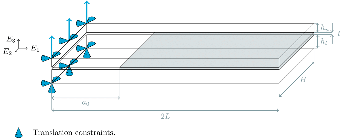
Here, the translation degrees of freedom parallel to the axis of the `blue cones are fixed. Additionally, the shaded region represents the cohesive zone interface while the unshaded region represents the bulk adherands or plies.`
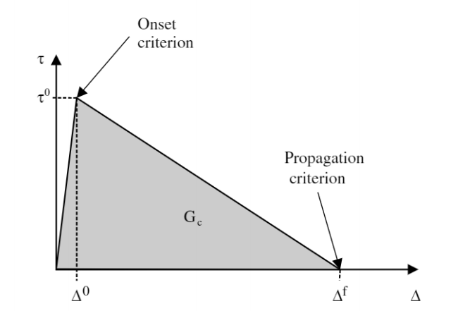
Fig. 5 Bilinear Traction Separation Law or the linear softening law [2].
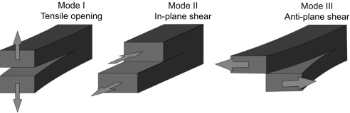
Interfaces tend to have different properties for opening (mode-I) and shear modes (mode-II and mode-III) in Fig. 6 , resulting in different traction separation laws represented above using subscripts `I for opening mode and sh for shear modes for the parameters.`
References:
Mudunuru, N. (2022, March 30). Finite Element Model For Interfaces In Compatibilized Polymer Blends. TU Delft Education Repositories. Retrieved on April 21, 2022, from http://resolver.tudelft.nl/uuid:88140513-120d-4a34-b893-b84908fe2373
Turon, A., Camanho, P., Costa, J., & Davila, C. (2006). A damage model for the simulation of delamination in advanced composites under variable-mode loading. Mechanics of Materials, 38(11), 1072–1089. https://doi.org/10.1016/j.mechmat.2005.10.003
Oterkus, E., Diyaroglu, C., de Meo, D., & Allegri, G. (2016). Fracture modes, damage tolerance and failure mitigation in marine composites. Marine Applications of Advanced Fibre-Reinforced Composites, 79–102. https://doi.org/10.1016/b978-1-78242-250-1.00004-1
LS-Dyna. (n.d.). Consistent units. Retrieved April 21, 2022, from https://www.dynasupport.com/howtos/general/consistent-units
Benzeggagh, M., & Kenane, M. (1996). Measurement of mixed-mode delamination fracture toughness of unidirectional glass/epoxy composites with mixed-mode bending apparatus. Composites Science and Technology, 56(4), 439–449. https://doi.org/10.1016/0266-3538(96)00005-x